Clustering Subreddit Communities

This project models Reddit user interactions to understand behavior and patterns. This project utilizes Spectral Clustering from the Graph Laplacian (using normalized cuts) to uncover local communities where users have more concentrated interactions. We discuss the importance of understanding user behavior, the results of this project, and areas of improvement for further research. If you’re interested, then let’s dive right in!

Reddit is a vast platform with countless communities, and understanding how these communities connect can provide valuable insights. For instance, knowing which Subreddits are often visited by the same users can help in creating better content recommendations, improving user engagement, or even in moderating content more effectively.

Contents

Here are the main sections of this article:

1. Loading the Data
2. Constructing the Graph Laplacian
3. K-Means Algorithm
4. Results and Observations
5. References

Loading the Data

The dataset was found on Kaggle and is called Subreddit Interactions for 25,000 Users. The dataset contains three columns: “user”, “subreddit”, and “utc-stamp”. For our analysis, we are only interested in the first two columns.

Before we start, we need to set up some libraries for our analysis and load in our data (Note: throughout this article, I will not be showing the subreddit names too often as far too many of them are NSFW!).

import numpy as np
import pandas as pd
import networkx as nx
from wordcloud import WordCloud
import matplotlib.pyplot as plt
%matplotlib inline
from sklearn.cluster import KMeans
from tqdm.notebook import tqdm
import os

interactions = pd.read_csv('reddit_data.csv').iloc[:, :-1]  # remove utc times
interactions.tail()

Preprocessing the Data

Now that we have our data loaded in, we need to somehow standardize user interactions so that one user does not have greater influence than another user. The approach outlined in the code below groups the interactions by username and finds the proportion of visits made by a user on specific subreddits. Here’s the mathematical formulation of this problem:

Given a dataset of interactions where each interaction is defined by a ‘username’ and a ‘subreddit’, we want to compute the probability of a user interacting with a specific subreddit.

Here, $n$ is the total number of interactions, $u_i$ is the $i$-th username, $s_i$ is the $i$-th subreddit in the dataset, and $r$ is the indicator function. Here is how we can implement this in Python efficiently:

subreddit_counts = interactions.groupby(['username', 'subreddit']).size().reset_index(name='subreddit_count')
total_counts = interactions.groupby('username').size().reset_index(name='total_count')
merged_df = pd.merge(subreddit_counts, total_counts, on='username')
merged_df['probabilities'] = merged_df['subreddit_count'] / merged_df['total_count']
interactions = pd.merge(interactions, merged_df[['username', 'subreddit', 'probabilities']], on=['username', 'subreddit'], how='left').values

del subreddit_counts, total_counts, merged_df

interactions = np.vstack(tuple(set(map(tuple,interactions))))  # removing duplicate interactions
display(interactions[-5:])

Now we have converted interactions into a numpy array and added a third columns with the interaction proportions by user. The data now only contains unique rows because we do not need to model redundant edges in our matrix. With this, we can create some maps that will help construct our adjacency matrix and reduce the computational complexity for algorithms later in this project.

nodes = np.unique(interactions[:, 1])
nodes_map = {node: i for i, node in enumerate(nodes)}
reverse_map = {i: node for i, node in enumerate(nodes)}
print("Number of Subreddit pages:", nodes.shape[0])

Constructing the Graph Laplacian

With our data set up and ready to go, we can begin constructing a weighted Adjacency Matrix. In our case, let $A$ be an adjacency matrix where $A_{i, j}$ represents the weighted connection between node $i$ and node $j$. Nodes are mapped from pages using a mapping function $\text{nodes_map}$ such that $i = \text{nodes_map}(\text{page1})$ and $j = \text{nodes_map}(\text{page2})$. If you wish to skip all the math, you can click here.

For each user $u$, let $P_u$ be the set of pages visited by $u$, and let $p_1$ and $p_2$ be any two pages in $P_u$. Define the class probabilities associated with $p_1$ and $p_2$ as $c(p_1)$ and $c(p_2)$, respectively.

The Adjacency Matrix $A$ is defined as follows [2]: \(A_{i, j} = \sum_{u \in U} \sum_{\substack{p_1, p_2 \in P_u \ p_1 \neq p_2}} c(p_1) \cdot c(p_2)\)

Where:

• $U$ is the set of all unique users.
• $P_u$ is the set of pages visited by user $u$.
• $c(p_1)$ and $c(p_2)$ are the class probabilities for pages $p_1$ and $p_2$, respectively.
• $i = \text{nodes_map}(p_1)$ and $j = \text{nodes_map}(p_2)$.
• $A_{i, j}$ is incremented by the product of the class probabilities $c(p_1) \cdot c(p_2)$.

With $A$ defined, we must then remove any disconnected edges.

Define a mask vector $\mathbf{m}$ of length $n$ such that:

Here, $\mathbf{m}_i$ is $1$ if node $i$ has at least one connection, and $0$ if it has no connections.

The reduced adjacency matrix $A{\prime}$ is obtained by selecting only the rows and columns where $\mathbf{m}[i] = 1$:

The Degree Matrix $D$ is defined as follows [2]:

Given a reduced adjacency matrix $A{\prime}$ (obtained from the original adjacency matrix $A$ after removing isolated nodes), the normalized diagonal degree matrix $D$ is defined as:

The Graph Laplacian Matrix $L$ is defined as follows [1]:

Via the normalized cuts method [1], the Graph Laplacian can be defined as:

To make the matrix symmetrical we can simply do:

Computing top $k$ eigenvectors:

Given the eigenvalue decomposition for $L$:

Where:

• $L$ is symmetric.
• $\lambda_i$ are the eigenvalues, ordered such that $ \lambda_1 \leq \lambda_2 \leq \dots \leq \lambda_n $.
• $x_i$ are the corresponding eigenvectors.

The top $k$ eigenvectors then become:

Implementing the Algorithm

With all the math aside, we can now create and run our algorithm!

A = np.zeros(shape=(nodes.shape[0], nodes.shape[0]), dtype=np.float32)

for u in tqdm(np.unique(interactions[:, 0])):
    users = interactions[interactions[:, 0] == u, 1:]
    
    for ind, page1 in enumerate(users[:-1]):
        i = nodes_map[page1[0]]
        for page2 in users[ind:]:
            j = nodes_map[page2[0]]
            if page1[0] != page2[0]:
                A[i, j] += page1[1].astype(np.float32) * page2[1].astype(np.float32)

A = A + A.T

mask = np.sum(A, axis=1) != 0
A = A[mask][:, mask]

D = np.diag(1/np.sqrt(np.sum(A, axis=1)))

L = D @ A @ D  # Graph Laplacian via Normalized Cuts method [1]
v, x = np.linalg.eigh(L)

print(f"A.shape: {A.shape}")
print(f"D.shape: {D.shape}")
print(f"L.shape: {L.shape}")
print(f"x.shape: {x.shape}")

Since the computation of the eigenvalue decomposition is extremely time-consuming, we can save the eigenvalue decomposition matrix with the code below.

eigs = os.path.join(os.getcwd(), f'GL_Eigenvectors_Weighted')
os.makedirs(eigs, exist_ok=True)
np.save(os.path.join(eigs, 'eigenvectors_x.npy'), x)

K-Means Algorithm

With our eigenvectors matrix computed, we can apply the k-means algorithm on this new dataset. Because of the nature of the Graph Laplacian, the data will naturally separate at weak edges, which creates local communities in the data. If you wish to skip all the math, you can click here.

The k-means algorithm aims to solve [2]:

Given $m$ data points $x^i \in \mathbb{R}^n, i = 1, . . . , m$, K-means clustering algorithm groups them into $k$ clusters by minimizing the function over ${r^{ij},\mu^j}.$

where $r^{ij} = 1$ if $x^i$ belongs to the $j$-th cluster and $r^{ij} = 0$ otherwise.

Once the minimization of the function over ${r^{ij},\mu^j}.$ is solved,

\(\mu^j = \frac{\sum_{i=1}^m r^{ij} x^i}{\sum_{i=1}^m r^{ij}}\) \(r^{ij} = \begin{cases} 1 & if \>\> j = \underset{j=1,...,k}{\operatorname{arg min}} \lVert x^i − c^j \lVert^2 \\ 0 & if \>\> j \neq \underset{j=1,...,k}{\operatorname{arg min}} \lVert x^i − c^j \lVert^2 \end{cases}\)

Implementing K-Means for Spectral Clustering

Let’s now implement the algorithm to find $k$ communities.

k = 1000

X = x[:, -k:]
labels = KMeans(n_clusters=k, n_init='auto').fit(X.real).labels_  # kmeans centers

labs = np.unique(labels)

clusters = []
lengths = []
for c in tqdm(labs):
    inds = np.where(labels == c)[0]
    cluster = {}
    
    for i in inds:
        if reverse_map[i] in cluster:
            cluster[reverse_map[i]] += 1
        else:
            cluster[reverse_map[i]] = 1
            
    clusters.append(cluster)
    lengths.append(len(cluster))
    
groups = pd.DataFrame({"Cluster": labs, "Subreddits": clusters, "Cluster Size": lengths}).sort_values(by="Cluster Size", ascending=False)
del clusters, cluster

results = pd.DataFrame({"Cluster": labels, "Subreddit": [reverse_map[i] for i in range(len(labels))]}).sort_values(by="Subreddit", ascending=False)

display(groups.head(), results.head())

Results and Observations

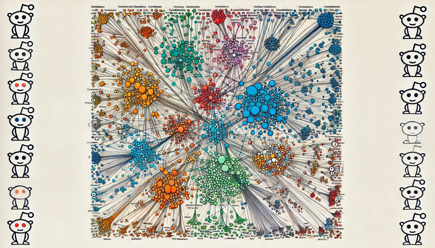
To understand how the spectral clustering algorithm performed, we can visualize two of the clusters to understand their relatedness to eachother. I had to run the algorithm several times because there were way too many NSFW Subreddits showing up!

top_percent_index = int(len(groups) * 0.02)

random_indices = np.random.choice(np.arange(1, top_percent_index), size=2, replace=False)

for i in random_indices:
    subreddit_dict = groups.iloc[i]['Subreddits']
    cluster_nodes = list(subreddit_dict.keys())
    
    indices = [nodes_map[node] for node in cluster_nodes if node in nodes_map]
    subgraph = nx.from_numpy_array(A[np.ix_(indices, indices)])
    subgraph = nx.relabel_nodes(subgraph, {i: reverse_map[i] for i in indices})
    edge_weights = np.array([A[u, v] for u, v in subgraph.edges()])
    edge_weights = (edge_weights - edge_weights.min()) / (edge_weights.max() - edge_weights.min()) * 5
    
    wordcloud = WordCloud(width=800, height=400, background_color='black', colormap='OrRd').generate_from_frequencies(subreddit_dict)
    
    plt.figure(figsize=(10, 5))
    plt.imshow(wordcloud, interpolation='bilinear')
    plt.axis('off')
    plt.title(f"Cluster {groups.iloc[i]['Cluster']} (Size: {groups.iloc[i]['Cluster Size']})")
    plt.show()
    
    plt.figure(figsize=(12, 8))
    pos = nx.spring_layout(subgraph, seed=42)  # Positions for all nodes
    nx.draw(subgraph, pos, with_labels=False, node_color='red', edge_color='gray', width=np.log10(edge_weights+0.8), node_size=50, font_size=10)
    plt.title(f"Subcommunity Network for Cluster {groups.iloc[i]['Cluster']}")
    plt.show()
    
    print('\n\n')

While the Spectral Clustering approach has revealed clear community trends among subreddits, the presence of outlier subreddits suggests that there may be room for optimization, particularly in choosing the number of clusters ($k$). This could be due to either the complexity of user behavior or a suboptimal value of $k$. Additionally, the choice of using commenting activity as a measure of subreddit engagement, while useful, might not be the best indicator of true user interest. Future projects could explore other data features, like subreddit joins or upvotes, which might provide a more accurate representation of user behavior.

The computational expense of Spectral Clustering also raises the question of whether simpler algorithms could achieve similar results. While Spectral Clustering excels at capturing complex relationships, it might be worth exploring more straightforward models that could offer efficiency gains, especially for large-scale applications. Despite these considerations, the model’s ability to uncover nuanced community structures without relying on complex neural networks is a significant advantage, making it a promising tool for building unsupervised recommendation systems in the future.

References

[1] Jianbo Shi and J. Malik, “Normalized cuts and image segmentation,” in IEEE Transactions on Pattern Analysis and Machine Intelligence, vol. 22, no. 8, pp. 888-905, Aug. 2000, doi: 10.1109/34.868688.

[2] Xie, Yao, “Spectral Clustering.” Class lecture, Computational Data Analytics, Georgia Institute of Technology, Atlanta, GA. August 21, 2024.